Neural networks are quickly becoming the go-to algorithm for most machine learning tasks and are heralded as the main factor shaping the future of technology. This rise in popularity is mainly due to the increase in computing power since the concept of neural networks was first presented (circa 1960’s) and the exponential increase in the amount of data generated each day. The increased computing power has enabled the neural network algorithms to show off their power and yield impressive results on today’s massive datasets in a way that previous machine learning algorithms simply cannot.
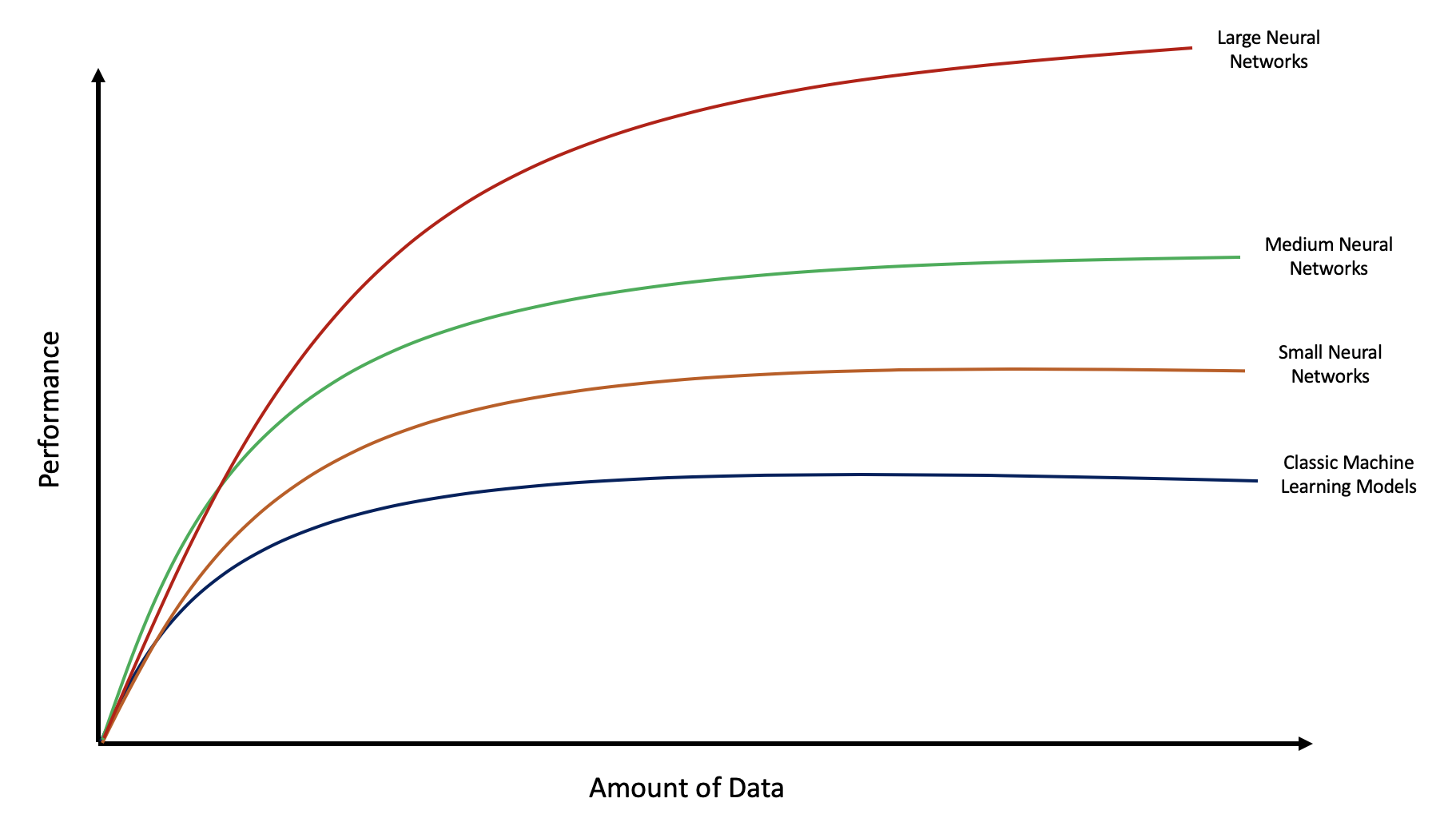
The figure below (based on a figure from Coursera’s Neural Network Specialization Series) illustrates how the quantity of available data is tied to model performance. The classic machine learning models tend to achieve their best performance measures with significantly less data than the other varying sizes of neural networks, but this performance plateaus at a lower level. As the size of the neural network gets larger, performance increases, but more data is needed to reach the plateau. The largest neural networks need the greatest amount of data to reach their superior performance measures, but this suggests that their performance then requires the greatest amount of time and computational power.
Despite their increased usage, neural networks have been categorized as “black box” models because we do not know exactly what is going on behind the scenes or what the network did to arrive at its prediction. We do, however, have a general idea of how the data moves through the network and this will be the focus of this first installment in my Neural Network Series. This post will give a generalized explanation of the structure and concepts underlying how neural networks work.
Biological Inspiration
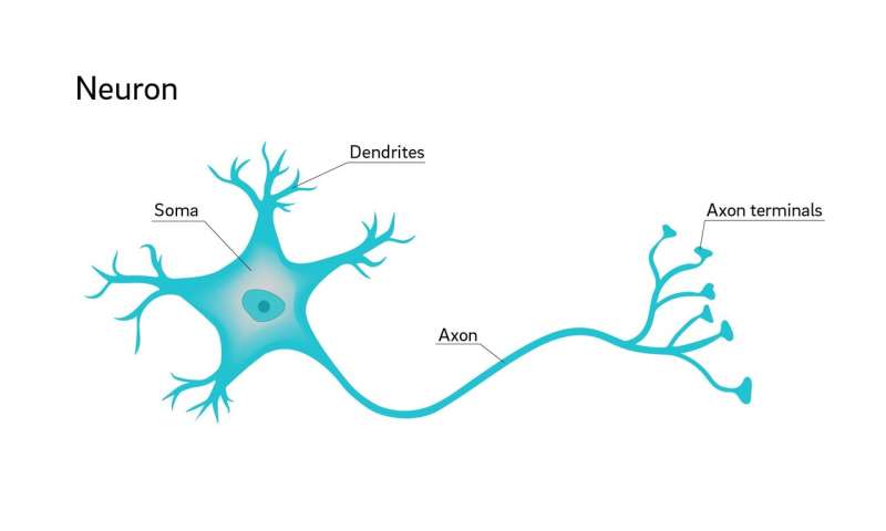
The building blocks of neural networks are called nodes. These nodes can be thought of (in both purpose and function) as the individual neurons that make up the human brain. The biological neuron depicted above has tiny projections (i.e. dendrites) where other neurons can connect with it to transfer information. The information collected from the other neurons is processed in the cell body (i.e. soma) and then sent down the axon via an action potential to the next neuron in the chain until it reaches the neurons in the region of the brain where it will ultimately be interpreted to form a decision/emotion/sensation.
The transfer of information within a neural network mimics the biological framework described above. The data is fed into the neural network at the input nodes. The input nodes process the data and then send it to the nodes in the next layer of the network, which then process and send the data to the next layer. The data continues to pass through the nodes of each layer until it reaches the output layer, where it is processed to generate a prediction.
General Architecture and Function

While there are different types of neural networks (which will be covered in a subsequent post), this post will focus on dense neural networks as they are the least complicated and therefore easiest to understand.
There are three main components in a dense neural network: the input layer, n number of hidden layers, and the output layer.
- Input Layer – where the data is fed into the neural network
- Hidden Layer(s) – groups of nodes applying mathematical transformations to the data as it moves through the layers of the neural network
- Linear: z = wx + b
- Activation Function = f(z)
- More on this in the next post!
- Output Layer – node(s) generating the prediction for the neural network
- Mathematical transformations happen in these nodes too
Mathematical Transformations
The linear transformation that occurs in the nodes of the neural network follows the equation z = wx + b, where w represents the weights and b represents the bias values. This can be likened to the “processing” that a biological neuron performs on the information it receives from other neurons.
The purpose of the activation function in the hidden layer nodes is to transfer the output of one node to the input of another node. These functions take the product of the linear transformation (z) as input and then yield some output based on the particular function used. In this sense, the activation function can be thought of as the action potential of biological neurons because it transfers the data from one node to the next down the chain. In the output layer nodes, the activation function produces the prediction.
Three Steps
The three steps that occur during each training iteration are: forward propagation, calculation of the loss and cost, and backward propagation.
- Forward Propagation – Applying mathematical transformations to the data as it moves through the neural network, ultimately to produce a prediction
- Calculation of Loss and Cost – Methods used to determine how wrong the neural network was compared to the ground-truth labels
- Loss – how far off the predicted value is from the ground-truth label for each training instance
- Cost – the average of the loss across all training instances
- Back Propagation – updating the weights (w) and bias values (b) for the nodes in the neural network based on gradient descent
Summary
The purpose of this post was to provide an introduction to neural networks and set the stage for more in-depth discussions of the concepts underlying their function that will come in subsequent installments of the Neural Network Series. I highly recommend exploring TensorFlow Playground to strengthen your understanding of how neural networks perform classification tasks before moving forward in this series. The next post will cover activation functions.