
The main goal of any machine learning model is to learn the classification/regression task from the data it was given. For models such as decision trees or random forests, “learning” happens in the form of finding the best way to successively split the data such that information gain is maximized (entropy is minimized) at each split. Neural networks, on the other hand, use an algorithm known as gradient descent to minimize the difference (loss) between the predicted and ground-truth values. As performing gradient descent involves calculating the partial derivative of the cost function with respect to each parameter in that function, it is a very computationally expensive process. This computational expense is also compounded by the massive amount of data neural networks need to achieve peak performance. Thus, many algorithms have been developed to improve upon the standard (stochastic) gradient descent such as Momentum, Root Mean Square Propagation (RMSProp), and Adaptive Moment Estimation (Adam).
In order to understand what optimizers might work best for a particular deep learning task, it is essential first to understand where optimizers fit into the neural network and how they participate in learning. Optimizers affect cost calculations and thereby affect how the weights and bias values are updated during backpropagation. Let’s briefly discuss back propagation before we dive into the specific optimizers.
Back Propagation
At this point the data has been fed forward through the network and it has generated a prediction. The loss (L(pred, true)) is calculated for each prediction based on how far off it is from its ground-truth value and then all of the loss measurements are averaged together to form a cost function (J(w,b)) for the entire network. The derivative of the cost function is calculated by taking the partial derivative with respect to each of its variables (w and b). The value of each variable’s derivative is used to update the weight and bias values throughout the network by multiplying the derivative by a learning rate and then subtracting this value from the current weight/bias value (i.e. updated w = current w - (alpha x dw)).
This is where the magic of gradient descent and its optimizers come into play. If the value of (alpha x dw) is negative, then the value of w will be updated in the positive direction. Whereas, if the value of (alpha x dw) is positive, the new value of w will be updated in the negative direction. The values of the weights/bias are updated in a direction opposite that of their derivative is because the cost function is convex (think U-shaped parabola). Since the derivative is the slope of the tangent line to the function and because we want to find the values for w (and b, but for the sake of explanation we will just focus on w for this example) that minimizes this cost function, we update their values based on what would bring them closer to the cost function minimum. Thus, if the derivative is positive, the w value is moving the function away from the minimum and it needs to be shifted in the negative direction, and vice versa.
What was just described above is stochastic gradient descent and it is effective at finding the minimum of the cost function given sufficient time. However, it is slow and can affect the efficiency of model production and deployment. The optimizers mentioned at the beginning of this discussion help speed convergence (finding the minimum of the cost function) along to address the efficiency issue of stochastic gradient descent.
Optimizers
Momentum
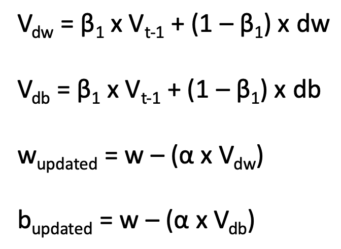
Adding momentum to stochastic gradient descent helps the algorithm converge faster because it utilizes a moving average of the previous gradient calculations to update the w and b values. With this method, the path towards convergence is more direct because the vertical oscillations have been reduced by the exponential weighted averages of the gradients.
The equation for applying momentum to stochastic gradient descent is shown below. It looks very similar to the equation for stochastic gradient descent, except that the exponentially weighted average of the gradient (V) is multiplied by the learning rate (alpha) instead of the derivative of w (or b, but again for the sake of explanation we will just focus on w). The beta parameter can be thought of as how many previous gradients are being included in the moving average. A larger beta indicates a greater number of previous gradients are included in the moving average, where a smaller beta indicates fewer gradients are included. The best way to determine beta for a project is through iterative training, but a value of 0.9 is a good place to start.
RMSProp
The RMSProp optimizer is very similar to adding momentum to stochastic gradient descent in that it reduces the vertical oscillations on the path to convergence. However, it does this by using the square of the current gradient instead of just the gradient. This is advantageous when using mini-batches (subgroups of the full training dataset) to train the network as is forces the gradient used in updates to be similar for adjacent mini-batches.
The equations for implementing RMSProp are shown below. Again, beta can be thought of as how many previous gradients to include in the same manner as with momentum (0.9 is still a good starting value). Epsilon is a correction parameter to ensure that we do not divide by zero when updating the weight and bias values. This parameter is usually set to 1e-9.
Adam
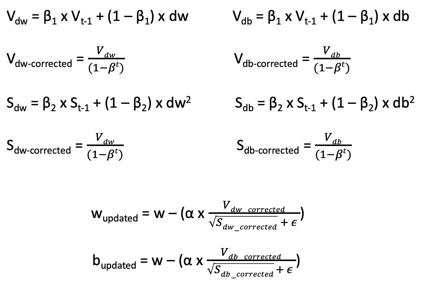
The Adam optimizer is essentially a combination of momentum and RMSProp. Thus, it has the efficiency advantages of momentum and the mini-batch performance increases seen with RMSProp. Because momentum and RMSProp reduce the vertical oscillations during gradient descent, the learning rate (alpha) may be able to be increased to speed up convergence. This combination of increased efficiency and performance is one of the main reasons the Adam optimizer is one of the most popular optimization algorithms used in the field of deep learning.
The equations to implement Adam are shown below. The beta values for the momentum-like portion and the RMSProp-like portion are different and the developers of the Adam optimizer suggest 0.9 and 0.999, respectively, as starting values. The epsilon value in the denominator of the RMSProp-like portion of the equation serves the same purpose as it does in the straight forward application of RMSProp and therefore should still be set to 1e-9. It is also important to note that when the Adam optimizer is used, the exponentially weighted average terms (V and S) undergo a bias correction calculation to minimize the effect of the randomly initialized values of V and S. These values are divided by 1 - beta^t (t being equal to the time step; number of gradients in the exponentially weighted moving average).
Summary
This post focused on how neural networks learn during back propagation and the optimization algorithms to make this learning more efficient. While the optimizers included in this post do not constitute an exhaustive list, the ones highlighted offer a discussion of the a few of the most popular algorithms used in the field of deep learning. Adding momentum to stochastic gradient descent accelerates convergence by reducing the magnitude of the oscillations in the vertical direction. RMSProp also reduces the magnitude of the vertical oscillations, but it does so by normalizing the magnitude of the step size, which makes this optimizer better when used with mini-batch training. Lastly, the Adam optimizer combines the benefits of momentum and RMSProp, making it a go-to choice for most neural network developers. As always, there is no way to truly know which optimizer will work best for a specific project besides trial and error, but the optimizers discussed in this post should provide an informed starting point for any deep learning project.
Additional Resources
Cost Functions and Gradient Descent
Video Lecture for Adam Optimizer
Why Correct for Bias in Adam Optimizer