As we collect more and more data as a society, we need more powerful tools to process it. This is where neural networks excel as they are able to handle high-dimensional data and complex processing with relatively little human intervention. While classic machine learning (ML) methods have been able to conquer classification and regression tasks such as filtering spam emails and predicting the price of an item, they do not perform well on natural language processing or image classification tasks. In essence, neural networks are being used to perform the complex tasks we ask our brains to do every day. For this reason, it is not surprising that the “under-the-hood” efforts of neural networks parallel (at a basic level) the processes of the neurons in our brain.
Understanding a Basic Neural Network
The basic neural network is known as the dense neural network. The term “dense” refers to how every neuron in one layer is connected to every neuron in the next layer throughout the model. The output of every neuron is connected to the next neuron by a weight, the value of which is optimized during back propagation via gradient descent. The figure below is an example of a dense neural network and the two sections that follow this figure outline the flow of data through it.

Step 1. Forward Propagation
For a dense neural network, the data is presented to an inner layer neuron (sometimes referred to a “hidden layer neuron/node/cell”), which transforms it with a linear function (weight * x + bias = z) to an output value (z) that is fed into an activation function. The activation function converts the output value z into the input value for the next neuron in the network or into the prediction if the neuron in in the last (output) layer of the network.
Step 2. Backward Propagation
The predicted value is compared to the ground truth value and a loss function is determined based on the difference between these two values. The derivative of the loss function is used with gradient descent to alter the values of the weights and biases in the neuronal linear transformation equations by going backwards through the layers of the network. Then new data is sent through the network to begin forward propagation again with the updated weights and biases until the overall cost function is minimized (best values for the weights and biases have been learned).
Extension to Recurrent Neural Networks

While most neural networks perform better than other ML models on natural language processing and image classification tasks, recurrent neural networks are a particular class of neural networks that perform exceedingly well on tasks where the sequence of the data is an important feature (e.g. time series analysis and natural language processing tasks). This is due to how the neurons of these networks evaluate the data as observations in time, rather than simply as individual observations.
For recurrent neural networks, a datapoint (x_1) enters a hidden layer neuron where it is transformed with a linear function (weights_h1 * x + bias_h1 = z_1) similar to the process outlined for a dense neural network to produce an output value (z_1). When the next datapoint (x_2) is given to the hidden layer neuron, some of the information from x_1 was retained as the “hidden state” (a vector) of the neuron that is also fed to the linear transformation function. This is where recurrent neural networks differ from dense neural networks in that information from the previous datapoint is used during the processing of the subsequent datapoint. Thus, the network has more information about each datapoint (i.e. its history), which aids in the eventual prediction.
The (z_1) value is fed into the activation function to produce a prediction, which is used to determine a loss function similar to the basic neural network. However, the backward propagation step for a recurrent neural network is a little different in that the weights and biases are updated by time step for each neuron instead of for the neuron as a single unit. This means that the network starts with the most recent output to calculate the loss and then this value is sent backwards through each time step to adjust the weights and biases.
While retaining some of the information from the previous datapoints seen by the neurons in the network ultimately aids its predictive capability, this adds to the computational expense of the network. Additionally, neurons in the earlier layers can become saturated and suffer the effects of a vanishing gradient. A vanishing gradient occurs during backwards propagation where the updates to the weights and biases become smaller and smaller as the propagation moves towards the early layers in the network. If insignificant changes are made to the weights and biases of the neurons in the earlier layers, they stop learning new information from the data. Thankfully, two special types of neurons have been created the get around the issues of saturation and the vanishing gradient, Long Short-Term Memory (LSTM) cells and Gated Recurrent Units (GRU).
Special Recurrent Network Neurons
Both the LSTM cells and GRUs act like mini recurrent neural networks and function in a similar way to each other. They use an internal activation function to determine how much of the information from previous datapoints needs to be retained and what can be discarded. For example, consider the sentence “Justin studied in Germany during his Fall and Spring semesters of college in 2016. As a result, he speaks fluent …“. It can be reasonably inferred that the last word in the sentence should be “german.” However, to get to that prediction, the information regarding what semesters and what year Justin studied in Germany did not add anything significant. Thus, they can be discarded and an accurate prediction for the end of the sentence can still be made. Similarly, LSTM cells and GRUs have the ability to update their internal state and actively discard bits of the sequence data that no longer contribute to the predictive capability of the network. While their approach to this differs slightly, they both function in forgetting information.
Long Short-Term Memory Cells
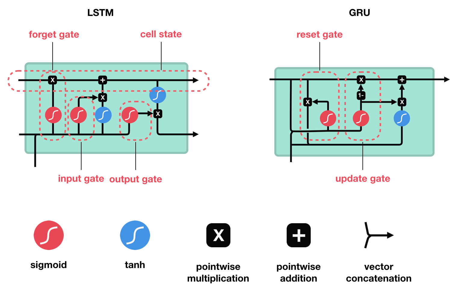
These cells were first introduced in 1997 by Sepp Hochreiter and Jurgen Schmidhuber. They contain three gates to update their internal state and determine what information to keep and what to forget:
- A Forget Gate, which decides what information can be discarded from the previous hidden state by combining it with the current datapoint input.
- An Input Gate, which decides what information is going to be retained from the current input datapoint. The internal cell state is updated by combining the outputs from the forget gate and the input gate.
- An Output Gate, which combines the previous hidden state, current datapoint input, and the updated internal cell state to produce the new hidden state (what information is carried to the next time step).
Gated Recurrent Units
These cells were first introduced in 2014 by Kyunghyun Cho. They work in a similar fashion to LSTM cells, except they replaced the internal cell state with the hidden state and only contain two gates:
- A Reset Gate, which decides how much of the previous information to discard.
- An Update Gate, which combines the functions of the forget an input gates from the LSTM cells. It decides what information from the current datapoint can be discarded and what should be added to the hidden state
Summary
This post was mean to be a high-level overview of the main topics concerning recurrent neural networks and their most recent advancements. While there was a lot of information presented, there are still significant areas that were touched on that require a deeper dive to fully understand the inner workings of these networks. I have included some helpful links at the end of this post to aid in the deeper dive. As for this post, the main take-aways are as follows:
- Neural networks typically perform better than classic ML models on natural language processing and image classification tasks.
- Recurrent neural networks are a class of neural networks that perform exceptionally well on sequence data as they retain information from previous time steps in the data sequence (e.g. they know where it has been to better predict where it is going).
- Recurrent neural networks are plagued by saturation and vanishing gradients where some of the layers stop learning new information from the data.
- Specialized cells for recurrent neural networks, LSTM and GRU, were developed to combat those issues and function in forgetting parts of the data sequence that do not contribute to the network’s predictive capability.
Additional Resources
This blog gives an overview of how neural networks differ from classic ML models
This blog give an excellent walk through of LSTM and GRU
- It also has an accompanying video walk-through of both recurrent neural networks and of LSTM/GRU